Classifying pictures of cats and dogs with Keras
The purpose of this notebook is to provide a quick demo of the ease-to-use of Keras.
We implement in a few dozens of lines a classifier for pictures of cats and dogs.
After several training epochs on 2x1024 pictures of cats and dogs, we obtain an accuracy of ~80% on the 2x416 pictures training set despite the small dataset size.
This noteboook goes along the blog post "Building powerful image classification models using very little data" written by François Chollet on blog.keras.io.
Overview :
- Data loading
- Model definition, training and evaluation
- Data augmentation
- Using a pre-trained network with bottleneck
Data
Data can be downloaded at: https://www.kaggle.com/c/dogs-vs-cats/data
Folder structure
data/
    train/
        dogs/ ### 1024 pictures
            dog001.jpg
            dog002.jpg
            ...
        cats/ ### 1024 pictures
            cat001.jpg
            cat002.jpg
            ...
    validation/
        dogs/ ### 416 pictures
            dog001.jpg
            dog002.jpg
            ...
        cats/ ### 416 pictures
            cat001.jpg
            cat002.jpg
            ...
Note : for this example we only consider 2x1000 training images and 2x400 testing images among the 2x12500 available.
Note 2 : this notebook require the Pillow framework to process images. You can install it using pip3 install Pillow
Data loading
from keras.preprocessing.image import ImageDataGenerator
# dimensions of our images.
img_width, img_height = 150, 150

train_data_dir = 'data/train'
validation_data_dir = 'data/validation'
# used to rescale the pixel values from [0, 255] to [0, 1] interval
datagen = ImageDataGenerator(rescale=1./255)

# automagically retrieve images and their classes for train and validation sets
train_generator = datagen.flow_from_directory(
        train_data_dir,
        target_size=(img_width, img_height),
        batch_size=32,
        class_mode='binary')

validation_generator = datagen.flow_from_directory(
        validation_data_dir,
        target_size=(img_width, img_height),
        batch_size=32,
        class_mode='binary')
Model
Imports
from keras.models import Sequential
from keras.layers import Convolution2D, MaxPooling2D
from keras.layers import Activation, Dropout, Flatten, Dense
Model architecture definition
model = Sequential()
model.add(Convolution2D(32, 3, 3, input_shape=(3, img_width, img_height)))
model.add(Activation('relu'))
model.add(MaxPooling2D(pool_size=(2, 2)))

model.add(Convolution2D(32, 3, 3))
model.add(Activation('relu'))
model.add(MaxPooling2D(pool_size=(2, 2)))

model.add(Convolution2D(64, 3, 3))
model.add(Activation('relu'))
model.add(MaxPooling2D(pool_size=(2, 2)))

model.add(Flatten())
model.add(Dense(64))
model.add(Activation('relu'))
model.add(Dropout(0.5))
model.add(Dense(1))
model.add(Activation('sigmoid'))
model.compile(loss='binary_crossentropy',
              optimizer='rmsprop',
              metrics=['accuracy'])
Training
nb_epoch = 1
nb_train_samples = 2048
nb_validation_samples = 832
model.fit_generator(
        train_generator,
        samples_per_epoch=nb_train_samples,
        nb_epoch=nb_epoch,
        validation_data=validation_generator,
        nb_val_samples=nb_validation_samples)
model.save_weights('models/1000-samples--1-epochs.h5')
Loading pre-trained model
model.load_weights('models/without-data-augmentation/1000-samples--32-epochs.h5')
Evaluating on validation set
Computing loss and accuracy :
model.evaluate_generator(validation_generator, nb_validation_samples)
Evolution of accuracy on training (blue) and validation (green) sets for 1 to 32 epochs :
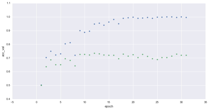
After ~10 epochs the neural network reach ~70% accuracy. We can witness overfitting, no progress is made over validation set in the next epochs
Data augmentation
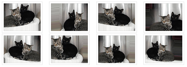
By applying random transformation to our train set, we artificially enhance our dataset with new unseen images.
This will hopefully reduce overfitting and allows better generalization capability for our network.
Example of data augmentation applied to a picture:
train_datagen_augmented = ImageDataGenerator(
        rescale=1./255,        # normalize pixel values to [0,1]
        shear_range=0.2,       # randomly applies shearing transformation
        zoom_range=0.2,        # randomly applies shearing transformation
        horizontal_flip=True)  # randomly flip the images

# same code as before
train_generator_augmented = train_datagen_augmented.flow_from_directory(
        train_data_dir,
        target_size=(img_width, img_height),
        batch_size=32,
        class_mode='binary')
model.fit_generator(
        train_generator_augmented,
        samples_per_epoch=nb_train_samples,
        nb_epoch=nb_epoch,
        validation_data=validation_generator,
        nb_val_samples=nb_validation_samples)
model.save_weights('models/1000-samples-augmented--1-epochs.h5')
model.load_weights('models/with-data-augmentation/1000-samples-augmented--100-epochs.h5')
Evaluating on validation set
Computing loss and accuracy :
model.evaluate_generator(validation_generator, nb_validation_samples)
Evolution of accuracy on training (blue) and validation (green) sets for 1 to 100 epochs :
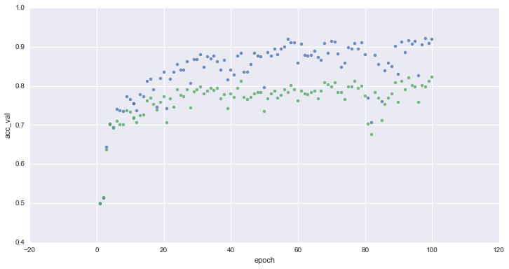
Thanks to data-augmentation, the accuracy on the validation set improved to ~80%
Using pre-trained model
The process of training a convolutionnal neural network can be very time-consuming and require a lot of datas.
We can go beyond the previous models in terms of performance and efficiency by using a general-purpose, pre-trained image classifier.
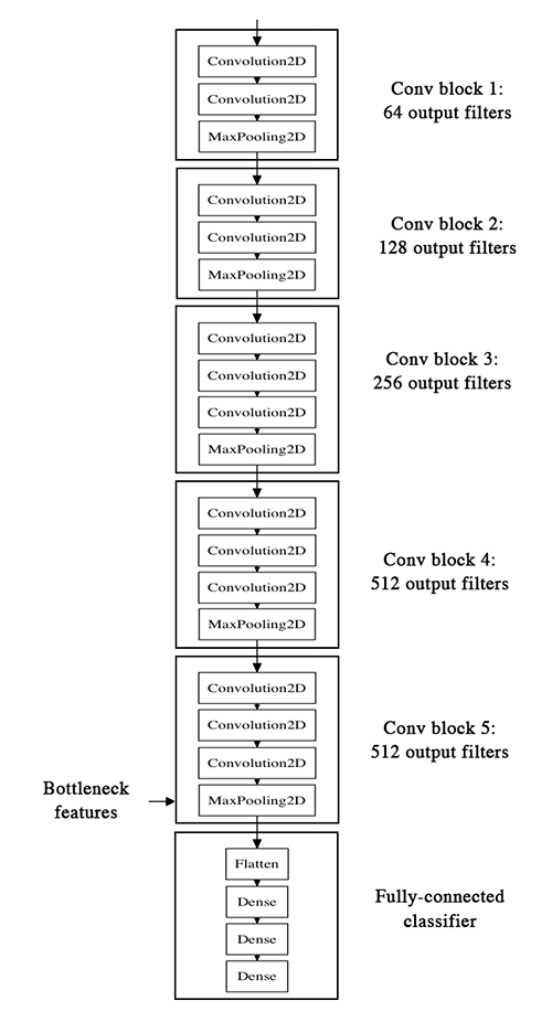
We consider VGG16, a model trained on the ImageNet dataset - which contains millions of images classified in 1000 categories.
On top of it, we add a small multi-layer perceptron and we train it on our dataset.
VGG16 + small MLP
VGG16 model architecture definition
import os
import numpy as np
from keras.preprocessing.image import ImageDataGenerator
from keras.models import Sequential
from keras.layers import Convolution2D, MaxPooling2D, ZeroPadding2D
from keras.layers import Activation, Dropout, Flatten, Dense
model_vgg = Sequential()
model_vgg.add(ZeroPadding2D((1, 1), input_shape=(3, img_width, img_height)))

model_vgg.add(Convolution2D(64, 3, 3, activation='relu', name='conv1_1'))
model_vgg.add(ZeroPadding2D((1, 1)))
model_vgg.add(Convolution2D(64, 3, 3, activation='relu', name='conv1_2'))
model_vgg.add(MaxPooling2D((2, 2), strides=(2, 2)))

model_vgg.add(ZeroPadding2D((1, 1)))
model_vgg.add(Convolution2D(128, 3, 3, activation='relu', name='conv2_1'))
model_vgg.add(ZeroPadding2D((1, 1)))
model_vgg.add(Convolution2D(128, 3, 3, activation='relu', name='conv2_2'))
model_vgg.add(MaxPooling2D((2, 2), strides=(2, 2)))

model_vgg.add(ZeroPadding2D((1, 1)))
model_vgg.add(Convolution2D(256, 3, 3, activation='relu', name='conv3_1'))
model_vgg.add(ZeroPadding2D((1, 1)))
model_vgg.add(Convolution2D(256, 3, 3, activation='relu', name='conv3_2'))
model_vgg.add(ZeroPadding2D((1, 1)))
model_vgg.add(Convolution2D(256, 3, 3, activation='relu', name='conv3_3'))
model_vgg.add(MaxPooling2D((2, 2), strides=(2, 2)))

model_vgg.add(ZeroPadding2D((1, 1)))
model_vgg.add(Convolution2D(512, 3, 3, activation='relu', name='conv4_1'))
model_vgg.add(ZeroPadding2D((1, 1)))
model_vgg.add(Convolution2D(512, 3, 3, activation='relu', name='conv4_2'))
model_vgg.add(ZeroPadding2D((1, 1)))
model_vgg.add(Convolution2D(512, 3, 3, activation='relu', name='conv4_3'))
model_vgg.add(MaxPooling2D((2, 2), strides=(2, 2)))

model_vgg.add(ZeroPadding2D((1, 1)))
model_vgg.add(Convolution2D(512, 3, 3, activation='relu', name='conv5_1'))
model_vgg.add(ZeroPadding2D((1, 1)))
model_vgg.add(Convolution2D(512, 3, 3, activation='relu', name='conv5_2'))
model_vgg.add(ZeroPadding2D((1, 1)))
model_vgg.add(Convolution2D(512, 3, 3, activation='relu', name='conv5_3'))
model_vgg.add(MaxPooling2D((2, 2), strides=(2, 2)))
Loading VGG16 weights
This part is a bit complicated because the structure of our model is not exactly the same as the one used when training weights.
Otherwise, we would use the model.load_weights() method.
Note : the VGG16 weights file (~500MB) is not included in this repository. You can download from here :
https://gist.github.com/baraldilorenzo/07d7802847aaad0a35d3
import h5py
f = h5py.File('models/VGG16/vgg16_weights.h5')

for k in range(f.attrs['nb_layers']):
    if k >= len(model.layers):
        # we don't look at the last (fully-connected) layers in the savefile
        break
    g = f['layer_{}'.format(k)]
    weights = [g['param_{}'.format(p)] for p in range(g.attrs['nb_params'])]
    model_vgg.layers[k].set_weights(weights)
f.close()
Using the VGG16 model to process samples
train_generator_bottleneck = datagen.flow_from_directory(
        train_data_dir,
        target_size=(img_width, img_height),
        batch_size=32,
        class_mode=None,
        shuffle=False)

validation_generator_bottleneck = datagen.flow_from_directory(
        validation_data_dir,
        target_size=(img_width, img_height),
        batch_size=32,
        class_mode=None,
        shuffle=False)
This is a long process, so we save the output of the VGG16 once and for all.
bottleneck_features_train = model_vgg.predict_generator(train_generator_bottleneck, nb_train_samples)
np.save(open('models/bottleneck_features_train.npy', 'wb'), bottleneck_features_train)
bottleneck_features_validation = model_vgg.predict_generator(validation_generator_bottleneck, nb_validation_samples)
np.save(open('models/bottleneck_features_validation.npy', 'wb'), bottleneck_features_validation)
Now we can load it...
train_data = np.load(open('models/bottleneck_features_train.npy', 'rb'))
train_labels = np.array([0] * (nb_train_samples // 2) + [1] * (nb_train_samples // 2))

validation_data = np.load(open('models/bottleneck_features_validation.npy', 'rb'))
validation_labels = np.array([0] * (nb_validation_samples // 2) + [1] * (nb_validation_samples // 2))
And define and train the custom fully connected neural network :
model_top = Sequential()
model_top.add(Flatten(input_shape=train_data.shape[1:]))
model_top.add(Dense(256, activation='relu'))
model_top.add(Dropout(0.5))
model_top.add(Dense(1, activation='sigmoid'))

model_top.compile(optimizer='rmsprop', loss='binary_crossentropy', metrics=['accuracy'])
nb_epoch=10
model_top.fit(train_data, train_labels,
          nb_epoch=nb_epoch, batch_size=32,
          validation_data=(validation_data, validation_labels))
The training process of this small neural network is very fast : ~2s per epoch
model_top.save_weights('models/1000-samples-bottleneck--10-epochs.h5')
Bottleneck model evaluation
model_top.load_weights('models/with-bottleneck/1000-samples--100-epochs.h5')
Loss and accuracy :
model_top.evaluate(validation_data, validation_labels)
Evolution of accuracy on training (blue) and validation (green) sets for 1 to 32 epochs :
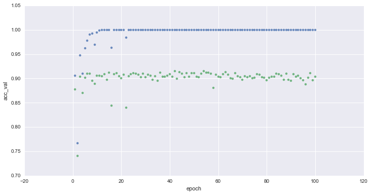
We reached a 90% accuracy on the validation after ~1m of training (~20 epochs) and 8% of the samples originally available on the Kaggle competition !